Predictive Solutions Series - Forecasting Module and Tool kit

Trusts and healthcare providers are under more pressure to plan and assess what the demand on the service is going to be in the future. The traditional reactive way of ‘firefighting’ is no longer an option, thus trusts and healthcare providers are being encouraged to: plan their capacity better, which can be done by using a future projection of what the demand is and to have forward looking information at their fingertips. This is the problem that this model solves.

Our forecasting tool gives trusts the opportunity to:

• Be prospective in their approach, allowing trusts and providers to future plan and be more proactive in their planning, by subsequent alignment of capacity to meet demand;
• Embed forecasting tool sets, into their daily business, to allow for the earlier identification of problem areas and pinch points;
• The ability to forecast over days, months and years. This forecast horizon can be configured to suit the needs of the service;
• Greater visibility of what there is to come, instead of what has already happened – looking through the drivers window, instead of the rear view mirror.

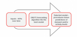
This model looks at five of the leading uni-variate forecasting models and chooses the model with the best fitting accuracy. These models have been chosen to work with any time horizon. This is illustrated in the process below:

Our model uses a univariate forecasting approach to the forecasting of demand. What does our model do differently to other approaches used on the market? For any given time series (that is something measured over a time axis) – the model uses:

• Autoregressive Integrated Moving Averages (ARIMA) to model seasonality, trend and random noise in the underlying data;
• Trigonometric seasonality and Box Cox transformation with ARMA errors (known as TBATS) – this is the best fitting model, and is most useful of hourly and daily observations over time;
• Exponential smoothing – can work exceptionally well with hospital data, as it is excellent at assessing something called auto-correlation in the previous time points – we use a variance of exponential smoothing called Holts-Winters to detect trend and seasonality;
• Then, we have developed two custom approaches namely hybrid and ensembles – that use the benefit of multiple time series models. These are part of what makes our tool different to standard approaches.

Once our model has run – it selects the best fitting model for the time series in question. It does this by using a well known metric called mean absolute percentage error (MAPE). This metric is calculated and then the model with the lowest MAPE is selected – for example we run the model on referral demand into an outpatient setting > 5 models run and fit a forecast line to the retrospective points > these points are extended forward by the given horizon > the model computes the errors between the predictions and the actual values > the MAPE is calculated and then the model juxtaposes the 5 models and chooses the lowest MAPE. Basically, MAPE is a measure of overall model prediction accuracy.

An additional feature of the model is that it partitions the time series into a ML partitioning approach, by splitting the data into train and test samples. The model is then trained on the time series using the training sample.

Once trained, the test data is used to generate predictions. In this way – the test data represents unseen values; these act like future values for assessing how well the model will perform in a ‘real world’ production environment and with real data.

The model is then assessed to see how accurate the test and training samples are, by doing this, we can show that the model might train well on the known retrospective values, but with future data – the model may not perform as well. This is another feature we use in our modelling process and it’s baked into our product.

D&D’s solutions are platform agnostic – meaning that we build the algorithms in isolation of any BI tool. This is advantageous, as it allows the integration into any BI application. The type of chart it would create in our native programming language R is below:

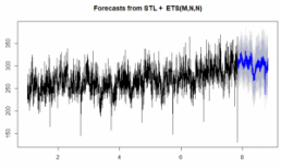
Our tool would provide additional outputs:

• Forecasted future values – based on the future horizon chosen – this could be 1 week, 1 month, 1 year, etc.
• Information on the model accuracy of the fitted model
• If forecasting a single indicator over multiple sites / specialties – then this would be each site or specialties forecast by the inputted indicator type e.g. GP referral demand by specialty

These outputs could be easily integrated into other solutions.